The Optics Laboratory

Group of Hans Hallen, North Carolina State University Physics Department

Feedback Theory

• General Considerations

• Gain & Phase vs. Frequency

• Example

• Alignment

Feedback loop:

• Digital

- Found on most commercial systems. - advantages: can 'guess' the offset needed for the next line so demand less from the feedback response. easier to achieve optimal frequency response. - disadvantages: can get noise from computer into the measurement system if not careful

• Analog

- Found on most home-made systems. - advantages relatively easy to build and get working immune to computer crashes

Feedback loop general concepts

• Pick a point on the approach curve to feedback on. (Say 1/2 the oscillation magnitude when the tip is far from the sample.)

• The detector output voltage and the setpoint voltage are fed into a differential amplifier to yield an error signal.

• The error signal is amplified by the feedback amplifier (analog or digital, gain = Gfb) and the output sent to drive the z-piezo element (fine approach control).

• This drives the tip until some equilibrium is established.

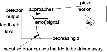
• The equilibrium is: Verror Gfb = Vz-piezo

• To minimize Verror hence positioning error - make Gfb bigger (this tends to cause stability problems -- addressed later) - make Vz-piezo smaller (use coarse approach) - trick feedback into thinking Vz-piezo smaller manually apply an offset voltage to the z-piezo. use a computer which sends the voltage used for the last line -- only small corrections should be needed.

• Stability is an important consideration.

• We want to estimate response time

• Gfb is always a function of frequency.

Linear feedback theory

• A schematic of our case:

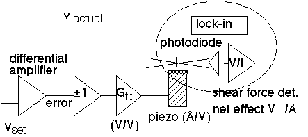
• This parallels what one would actually find in an instrument (except +/-1 may be moved some, I included the high voltage amplifiers in Gfb and I left off filters and where the computer is).

• The shear force detector depends on

- shear force light level.

- detecting efficiency (screen position, optics, etc.)

- the photodiode used.

- the current preamplifier gain.

- the lock-in amplifier settings.

- the slope of the approach curve (which in turn depends upon the sample).

• We assume linearity here.

- O.K. for small excursions from the set point.

- Interferometry method is linear in phase difference (but approach curve may not be).

• Compare shear force det. to STM current det. -- exponential

• Putting it into one pot

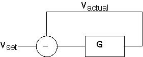
• A simple relation follows:

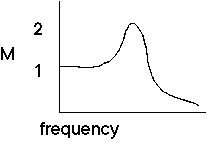
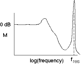
• And the closed loop gain M

• For M = 1, want G >> 1

• Recall G has a phase and eventually (as w gets large) approaches zero.

- Problems if G = -1 ( |G| = 1 w/ 180° phase)

• Reference:

- Feedback Control Systems, John Van de Vegte (Prentice Hall).

• Closed loop gain

• Plot on computer or sketch.

• Example: underdamped resonance.

Estimating what parts of G(w) may look like:

• G(w) = G1(w) * G2(w) * G3(w) * ...

(1)For a single pole roll-off

- model as a resistor and capacitor

- although more complicated amplifier circuits will behave the same way.

- The gain magnitude is , and the phase is - arctan(wRC)

- The gain magnitude falls at the rate of 6dB/octave = 20dB/decade of frequency at high frequencies (i.e., proportional to 1/w). G (dB) = 20 log(G(voltage ratio))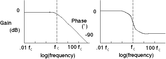

- get 90° of phase shift from a single pole.

- for a double pole, get 180° of phase which can be bad news if |G| near 1.

(2)An electro-mechanical system, the piezo's

- have mechanical resonances

- can calculate them from the formulas above: for typical sizes, lowest resonance might be a few 10's of kHz.

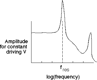
- Very high scan-rate (feedback bandwidth) microscopes have to face this unless the mechanics are carefully designed to eliminate (push to higher frequency) or damp the resonances.

- possible result:

(3) We want to estimate the gain magnitude and phase for each component of the feedback loop, keeping a special eye on the phase (which comes over a broad range, 90° at frequencies far above the pole frequency).

• Consider:

- any electronics. Usually it is easy to pick components such that these have flat G with little phase (high gain: watch the gain- bandwidth product limitations).

- photodiode: RC roll-off from current pre- amplifier.

- Lock-in amplifier: RC set by the time constant roll-off rate can also be controlled (#of poles) Should always be set to 6dB/octave.

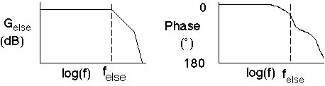
- Gfb: this is where we try to fix things up.

• Lump all the components but Gfb into Gelse

• A possible case:

Tuning the feedback loop.

• This discussion presumes that a well- constructed, properly aligned microscope is being used. Also that a good clean sample and tip are in place. Otherwise, Gelse may have some strange features not considered here.

• We will use the Gelse given above and a Gfb typical of what is used for scanning probes: a proportional-integral feedback, shown below.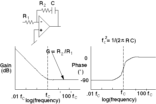

• The PI has gain magnitude and phase given by .

• The integral part gives high gain at low frequencies for accuracy (low error voltage).

• The proportional part allows us to extend the loop frequency range in those cases where the Gelse part has a region with only a single pole roll-off (to go through Gloop=1 with). If Gelse has a double pole roll-off right away, then it will be tricky to get a stable loop unless the integral part is used to bring Gloop through 1 while Gelse is still flat. The proportional part is turned down to allow Gloop to pass through 1, although one may wish to keep 1/(2pR2C) close to provide a little help with the phase (note it pushes the phase less negative, so compensates for other phase from Gelse).

• We are aiming to achieve the following Gloop: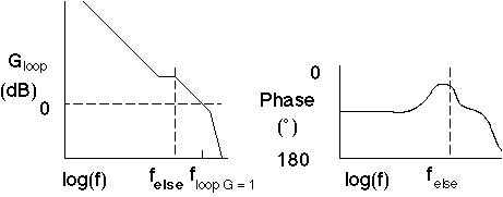

• First the integral gain is turned up until oscillations occur. This is when two poles are present near Gloop = 1, i.e., near felse. Turn the integral gain down until the oscillations stop.

• Now the proportional gain is increased until oscillations occur. This is near where Gelse is falling by 12 dB/octave. Turn the proportional gain down until the oscillations stop.

• The coarse alignment is finished. Now the final tuning begins.

• Apply a small square wave to either the z-piezo voltage or the requested Vset. Either will force the feedback loop to correct for the perturbation.

• We are aiming for:

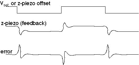
• If ringing is seen on the error voltage, reduce the gains (try proportional first).

• If the error voltage approaches zero very slowly with no overshoot, increase the gains (integral first).

• Note that the best you can do (slight overshoot) may seem to have a slow time constant. The solution is to find the object responsible for the low frequency drop in Gelse and speed it up.

• Tuning depends on the slope of the approach curve, and the position on that curve (Gelse changes)

• If there is too much noise in the system, you may have to slow the loop down, but a good microscope and clean sample and tip should make this unnecessary.

• How fast can you scan?

- You know G(w) from the aim-for plot above and the settings (also felse and what settings it oscillated at).

- Use . This is 1/2 at G = 1 (so a factor of 2 error), but is 0.91 at G=10.

- Decide on your accuracy and set speed. On rough surfaces, you may need to slow down so that the tip doesn't crash on the way. Speed may also be limited by optical signal considerations.

- Experimentally, look at the response during fine-tuning.

• References:

- several articles in IBM J. Res. Develop. 30 (1986).

Feedback in the Presence of Nonlinearities

• Tapping is nonlinear:

- The force abruptly increases at the point when the probe encounters the surface.

- There is a frequency shift.

• The response depends upon direction:

- When retracting from the surface, the probe amplitude decreases with time constant related to the inverse peak bandwidth. (This is why we see it with tuning forks — the width is low enough that it is a problem.)

- When approaching the surface, the nonlinear force quickly quenches the motion.

- This leads to low frequency oscillations.

• Use the nonlinearity to fix it:

- Set the feedback frequency lower than the peak (with retracted tip).

- As feedback is engaged, the peak shifts to higher frequencies, rapidly reducing the level at the operating frequency.

- Now, when retracting from the surface, the level at the operating frequency increases due to the resonance peak shifting back.

- Note: the magnitude of this effect depends upon the slope of the resonance curve at the operating frequency (steeper means more response). Choose frequency so that the speeds in-and-out are the same. Use forward-reverse scanning.

North Carolina State University | Physics | Optics Home